
自由软件工程师
Jan is a business intelligence and data warehousing expert with advanced R skills and some infrastructure experience.
Jan is a business intelligence and data warehousing expert with advanced R skills and some infrastructure experience.
The R language is often perceived as a language for statisticians and data scientists. Quite a long time ago, this was mostly true. However, over the years the flexibility R provides via packages has made R into a more general purpose language. R was open sourced in 1995, and since that time repositories of R packages are constantly growing. Still, compared to languages like Python, R is strongly based around the data.
说到数据, tabular data deserves particular attention, as it’s one of the most commonly used data types. 它是一种数据类型,对应于数据库中已知的表结构, where each column can be of a different type, and processing performance of that particular data type is the crucial factor for many applications.

在本文中, we are going to present how to achieve tabular data transformation in an efficient manner. Many 使用R的人 already for machine learning are not aware that 数据绿豆 can be done faster in R, and that they do not need to use another tool for it.
以R为底引入了 data.frame class in the year 1997, which was based on S-PLUS before it. Unlike commonly used databases which store data row by row, R data.frame stores the data in memory as a column-oriented structure, thus making it more cache-efficient for column operations which are common in analytics. 另外, even though R is a functional programming language, it does not enforce that on the developer. Both opportunities have been well addressed by data.table R package, which is available in CRAN repository. It performs quite fast when grouping operations, and is particularly memory efficient by being careful about materializing intermediate data subsets, such as materializing only those columns necessary for a certain task. It also avoids unnecessary copies through its reference semantics while adding or updating columns. The first version of the package has been published in April 2006, significantly improving data.frame 当时的表现. The initial package description was:
This package does very little. The only reason for its existence is that the white book specifies that data.框架必须有行名. This package defines a new class data.table which operates just like a data.frame, but uses up to 10 times less memory, and can be up to 10 times faster to create (and copy). It also takes the opportunity to allow subset() and with() like expressions inside the []. Most of the code is copied from base functions with the code manipulating row.名字删除.
从那以后, data.frame and data.table implementations have been improved, but data.table remains to be incredibly faster than base R. In fact, data.table isn’t just faster than base R, but it appears to be one of the fastest open-source data wrangling tool available, 与诸如 Python熊猫, and columnar storage databases or big data apps like Spark. Its performance over distributed shared infrastructure hasn’t been yet benchmarked, but being able to have up to two billion rows on a single instance gives promising prospects. Outstanding performance goes hand-in-hand with the 功能. 另外, with recent efforts at parallelizing time-consuming parts for incremental performance gains, one direction towards pushing the performance limit seems quite clear.
Learning R gets a little bit easier because of the fact that it works interactively, so we can follow examples step by step and look at the results of each step at any time. Before we start, let’s install the data.table 包从CRAN存储库.
install.包(“数据.table")
有用的提示: We can open the manual of any function just by typing its name with leading question mark, i.e. ?install.packages.
There are tons of packages for extracting data from a wide range of formats and databases, which often includes native drivers. 中加载数据 CSV file, the most common format for raw tabular data. File used in the following examples can be found here. We don’t have to bother about CSV 阅读性能 fread function is highly optimized on that.
为了使用包中的任何函数,我们需要用 library call.
库(数据.table)
DT <- fread("flights14.csv")
print(DT)
##年月日dep_delay arr_delay载波原点dest air_time
## 1: 2014 1 1 14 13 aa肯尼迪国际机场359
## 2: 2014年1 1 -3 13 aa肯尼迪国际机场363
## 3: 2014年1 1 2 9 aa肯尼迪国际机场351
## 4: 2014 1 1 -8 -26 aa lga pbi 157
## 5: 2014年1 1 2 1 aa肯尼迪机场lax 350
##     ---
## 253312: 2014年10月31日1 -30日
## 253313: 2014年10月31日-5日-14日
## 253314: 2014 10 31 -8 16 mq lga rdu 83
## 253315: 2014 10 31 -4 15 mq lga DTW 75
## 253316: 2014 10 31 -5 1 mq lga SDF 110
##距离小时
##      1:     2475    9
##      2:     2475   11
##      3:     2475   19
##      4:     1035    7
##      5:     2475   13
##     ---
## 253312:     1416   14
## 253313:     1400    8
## 253314:      431   11
## 253315:      502   11
## 253316:      659    8
If our data is not well modeled for further processing, 因为它们需要从长到宽或从宽到长(也称为 pivot and unpivot)格式,我们可以看看 ?dcast and ?melt 函数,从 reshape2 package. However, data.table implements faster and memory efficient methods for data.table/data.框架类.
data.table Syntaxdata.frame
Query data.table 很像查询吗 data.frame. 在进行过滤时 i argument, we can use column names directly without the need to access them with the $ sign, like df[df$col > 1, ]. When providing the next argument j, we provide an expression to be evaluated in the scope of our data.table. 传递一个非表达式 j 参数使用 with=FALSE. Third argument, not present in data.frame method, defines the groups, making the expression in j 分组评估.
# data.frame
DF[DF$col1 > 1L, c("col2", "col3")]
# data.table
DT[col1 > 1L, .(col3 col2), ...] # by group using: `by = col4`
Query data.table in many aspects corresponds to SQL queries that more people might be familiar with. DT 下面的代表 data.table object and corresponds to SQLs FROM clause.
DT[i =其中,
    J = select | update
    [组]
  [ having, ... ]
  命令; ... ]
  [ ... ] ... [ ... ]

Sorting data is a crucial transformation for time series, and it is also imports for data extract and presentation. Sort can be achieved by providing the integer vector of row order to i 论证,和 data.frame. 查询中的第一个参数 订单(载体,-dep_delay) will select data in ascending order on carrier field and descending order on dep_delay measure. 第二个参数 j, as described in the previous section, defines the columns (or expressions) to be returned and their order.
ans <- DT[订单(载体,-dep_delay),
          .(carrier, origin, dest, dep_delay)]
head(ans)
##    carrier origin dest dep_delay
## 1:      AA    EWR  DFW      1498
## 2:      AA    JFK  BOS      1241
## 3:      AA    EWR  DFW      1071
## 4:      AA    EWR  DFW      1056
## 5:      AA    EWR  DFW      1022
## 6:      AA    EWR  DFW       989
To re-order data by reference, instead of querying data in specific order, we use set* functions.
setorder(DT, carrier, -dep_delay)
leading.cols <- c("carrier","dep_delay")
setcolorder (DT, c(领先.cols, setdiff(names(DT), leading.cols)))
print(DT)
##运营商dep_delay年月日arr_delay原点dest air_time
## 1: aa 1498 2014 10 4 1494 ewr DFW 200
## 2: aa 1241 2014 4 15 1223 JFK bos 39
## 3: aa 1071 2014 6 13 1064 ewr DFW 175
## 4: aa 1056 2014 9 12 1115 ewr DFW 198
## 5: aa 1022 2014 6 16 1073 ewr DFW 178
##     ---
## 253312: wn -12 2014 3 9 -21 lga bna 115
## 253313: wn -13 2014 3 10 -18 ewr MDW 112
## 253314: wn -13 2014 5 17 -30 lga hou 202
## 253315: wn -13 2014 6 15 10 lga mke 101
## 253316: wn -13 2014 8 19 -30 lga cak 63
##距离小时
##      1:     1372    7
##      2:      187   13
##      3:     1372   10
##      4:     1372    6
##      5:     1372    7
##     ---
## 253312:      764   16
## 253313:      711   20
## 253314:     1428   17
## 253315:      738   20
## 253316:      397   16
大多数情况下,我们不需要 both the original dataset and the ordered/sorted dataset. By default, R语言, similar to other functional programming languages, will return sorted data as new object, and thus will require twice as much memory as sorting by reference.
让我们为航班起点“JFK”和月份从6到9创建一个子集数据集. In the second argument, we subset results to listed columns, adding one calculated variable sum_delay.
ans <- DT[origin == "JFK" & 月%在% 6:9,
          .(origin, month, arr_delay, dep_delay, sum_delay = arr_delay + dep_delay)]
head(ans)
##    origin month arr_delay dep_delay sum_delay
## 1:    JFK     7       925       926      1851
## 2:    JFK     8       727       772      1499
## 3:    JFK     6       466       451       917
## 4:    JFK     7       414       450       864
## 5:    JFK     6       411       442       853
## 6:    JFK     6       333       343       676
By default, when subsetting dataset on single column data.table will automatically create an index for that column. 这导致 real-time answers on any further filtering calls on that column.
Adding a new column by reference is performed using the := operator, it assigns a variable into dataset in place. This avoids in-memory copy of dataset, so we don’t need to assign results to each new variable.
DT[, sum_delay := arr_delay + dep_delay]
head(DT)
##运营商dep_delay年月日arr_delay原点dest air_time
## 1: aa 1498 2014 10 4 1494 ewr DFW 200
## 2: aa 1241 2014 4 15 1223 JFK bos 39
## 3: aa 1071 2014 6 13 1064 ewr DFW 175
## 4:      AA      1056 2014     9  12      1115    EWR  DFW      198
## 5:      AA      1022 2014     6  16      1073    EWR  DFW      178
## 6:      AA       989 2014     6  11       991    EWR  DFW      194
##    distance hour sum_delay
## 1:     1372    7      2992
## 2:      187   13      2464
## 3:     1372   10      2135
## 4:     1372    6      2171
## 5:     1372    7      2095
## 6:     1372   11      1980
To add more variables at once, we can use DT[, :=(sum_delay = arr_delay + dep_delay)] 语法类似于 .(sum_delay = arr_delay + dep_delay) 从数据集查询时.
It is possible to sub-assign by reference, updating only particular rows in place, 仅仅通过结合 i argument.
DT[起源= =“肯尼迪”,
   距离:= NA]
head(DT)
##运营商dep_delay年月日arr_delay原点dest air_time
## 1: aa 1498 2014 10 4 1494 ewr DFW 200
## 2: aa 1241 2014 4 15 1223 JFK bos 39
## 3: aa 1071 2014 6 13 1064 ewr DFW 175
## 4:      AA      1056 2014     9  12      1115    EWR  DFW      198
## 5:      AA      1022 2014     6  16      1073    EWR  DFW      178
## 6:      AA       989 2014     6  11       991    EWR  DFW      194
##    distance hour sum_delay
## 1:     1372    7      2992
## 2:       NA   13      2464
## 3:     1372   10      2135
## 4:     1372    6      2171
## 5:     1372    7      2095
## 6:     1372   11      1980
To aggregate data, we provide the third argument by 到方括号. Then, in j we need to provide aggregate function calls, so the data can be actually aggregated. The .N 中使用的符号 j argument corresponds to the number of all observations in each group. As previously mentioned, aggregates can be combined with subsets on rows and selecting columns.
ans <- DT[,
          .(m_arr_delay = mean(arr_delay),
            m_dep_delay = mean(dep_delay),
            count = .N),
          .(载体、月)]
head(ans)
##    carrier month m_arr_delay m_dep_delay count
## 1:      AA    10    5.541959    7.591497  2705
## 2:      AA     4    1.903324    3.987008  2617
## 3:      AA     6    8.690067   11.476475  2678
## 4:      AA     9   -1.235160    3.307078  2628
## 5:      AA     8    4.027474    8.914054  2839
## 6:      AA     7    9.159886   11.665953  2802
Often, we may need to compare a value of a row to its aggregate over a group. 在SQL中,我们应用 划分上的聚合: AVG(arr_delay) OVER (PARTITION BY carrier, month).
ans <- DT[,
          .(arr_delay, carrierm_mean_arr = mean(arr_delay),
            dep_delay, carrierm_mean_dep = mean(dep_delay)),
          .(载体、月)]
head(ans)
##运营商月arr_delay carrier erm_mean_arr dep_delay carrier erm_mean_dep
## 1:      AA    10      1494          5.541959      1498          7.591497
## 2:      AA    10       840          5.541959       848          7.591497
## 3:      AA    10       317          5.541959       338          7.591497
## 4:      AA    10       292          5.541959       331          7.591497
## 5:      AA    10       322          5.541959       304          7.591497
## 6:      AA    10       306          5.541959       299          7.591497
If we don’t want to query data with those aggregates, and instead just put them into actual table updating by reference, 我们可以用 := operator. This avoids the in-memory copy of the dataset, so we don’t need to assign results to the new variable.
DT[,
   `:=`(carrierm_mean_arr = mean(arr_delay),
        carrierm_mean_dep = mean(dep_delay)),
   .(载体、月)]
head(DT)
##运营商dep_delay年月日arr_delay原点dest air_time
## 1: aa 1498 2014 10 4 1494 ewr DFW 200
## 2: aa 1241 2014 4 15 1223 JFK bos 39
## 3: aa 1071 2014 6 13 1064 ewr DFW 175
## 4:      AA      1056 2014     9  12      1115    EWR  DFW      198
## 5:      AA      1022 2014     6  16      1073    EWR  DFW      178
## 6:      AA       989 2014     6  11       991    EWR  DFW      194
##    distance hour sum_delay carrierm_mean_arr carrierm_mean_dep
## 1:     1372    7      2992          5.541959          7.591497
## 2:       NA   13      2464          1.903324          3.987008
## 3:     1372   10      2135          8.690067         11.476475
## 4:     1372    6      2171         -1.235160          3.307078
## 5:     1372    7      2095          8.690067         11.476475
## 6:     1372   11      1980          8.690067         11.476475
Base R数据集的连接和合并被认为是一种特殊类型的 subset operation. We provide a dataset to which we want to join in the first square bracket argument i. For each row in dataset provided to i, we match rows from the dataset in which we use [. If we want to keep only matching rows (inner join), then we pass an extra argument nomatch = 0L. We use on argument to specify columns on which we want to join both datasets.
#创建引用子集
carrierdest <- DT[, .(count=.N), .(carrier, dest) # count by carrier and dest
                  ][1:10                        # just 10 first groups
                    ]                           # chaining `[...][...’作为子查询
打印(carrierdest)
载波dest count
## 1: aa DFW 5877
## # 2: aa bo 1173
## 3: a ord 4798
## 4: aa sea 298
## 5: 85岁
## 6: aa lax 3449
## 7: aa mia 6058
## 8: aa sfo 1312
## 9: aa = 297
## 10: aa dca 172
#外连接
ans <- carrierdest[DT, on = c("carrier","dest")]
print(ans)
##运营商dest计数dep_delay年月日arr_delay起源
## 1: aa DFW 5877 1498 2014 10 4 1494 ewr
## 2: aa bos 1173 1241 2014 4 15 1223 JFK
## 3: aa DFW 5877 1071 2014 6 13 1064 ewr
## 4: aa DFW 5877 1056 2014 9 12 1115 ewr
## 5: aa DFW 5877 1022 2014 6 16 1073 ewr
##     ---
## 253312: wbna na -12 2014 3 9 -21 lga
## 253313: wn MDW na -13 2014 3 10 -18 ewr
## 253314:我的天哪-13 2014 5 17 -30 lga
## 253315: wmmake na -13 2014 6 15 10 lga
## 253316: wca na -13 2014 8 19 -30 lga
##         air_time distance hour sum_delay carrierm_mean_arr
##      1:      200     1372    7      2992          5.541959
##      2:       39       NA   13      2464          1.903324
##      3:      175     1372   10      2135          8.690067
##      4:      198     1372    6      2171         -1.235160
##      5:      178     1372    7      2095          8.690067
##     ---
## 253312:      115      764   16       -33          6.921642
## 253313:      112      711   20       -31          6.921642
## 253314:      202     1428   17       -43         22.875845
## 253315:      101      738   20        -3         14.888889
## 253316:       63      397   16       -43          7.219670
##         carrierm_mean_dep
##      1:          7.591497
##      2:          3.987008
##      3:         11.476475
##      4:          3.307078
##      5:         11.476475
##     ---
## 253312:         11.295709
## 253313:         11.295709
## 253314:         30.546453
## 253315:         24.217560
## 253316:         17.038047
#内连接
ans <- DT[carrierdest,                # for each row in carrierdest
          nomatch = 0L, #只返回两个表中匹配的行
          on = c("carrier","dest")]   # joining on columns carrier and dest
print(ans)
##运营商dep_delay年月日arr_delay原点dest air_time
## 1: aa 1498 2014 10 4 1494 ewr DFW 200
## 2: aa 1071 2014 6 13 1064 ewr DFW 175
## 3: aa 1056 2014 9 12 1115 ewr DFW 198
## 4: aa 1022 2014 6 16 1073 ewr DFW 178
## 5: aa 989 2014 6 11 991 ewr DFW 194
##    ---
## 23515: aa -8 2014 10 11 -13 JFK dca 53
## 23516: aa -9 2014 5 21 -12 JFK dca 52
## 23517: aa -9 2014 6 5 -6 JFK dca 53
## 23518: aa -9 2014 10 2 -21 JFK dca 51
## 23519: aa -11 2014 5 27 10 JFK dca 55
##距离小时sum_delay carrierm_mean_arr carrierm_mean_deep计数
##     1:     1372    7      2992          5.541959          7.591497  5877
##     2:     1372   10      2135          8.690067         11.476475  5877
##     3:     1372    6      2171         -1.235160          3.307078  5877
##     4:     1372    7      2095          8.690067         11.476475  5877
##     5:     1372   11      1980          8.690067         11.476475  5877
##    ---
## 23515:       NA   15       -21          5.541959          7.591497   172
## 23516:       NA   15       -21          4.150172          8.733665   172
## 23517:       NA   15       -15          8.690067         11.476475   172
## 23518:       NA   15       -30          5.541959          7.591497   172
## 23519:       NA   15        -1          4.150172          8.733665   172
Be aware that because of the consistency to base R subsetting, the outer join is by default 正确的外. 如果我们在寻找 LEFT OUTER, we need to swap the tables, as in the example above. Exact behavior can also be easily controlled in merge data.table method, using the same API as base R merge data.frame.
If we want to simply lookup the column(s) to our dataset, we can efficiently do it with := 运营商 j 加入时的争论. The same way as we sub-assign by reference, as described in the 更新数据集 section, we just now add a column by reference from the dataset to which we join. This avoids the in-memory copy of data, so we don’t need to assign results into new variables.
DT[carrierdest,                     # data.连接表
   lkp.Count:= Count, #从' carrier '中查找' Count '列
   on = c("carrier","dest")]        # join by columns
head(DT)
##运营商dep_delay年月日arr_delay原点dest air_time
## 1: aa 1498 2014 10 4 1494 ewr DFW 200
## 2: aa 1241 2014 4 15 1223 JFK bos 39
## 3: aa 1071 2014 6 13 1064 ewr DFW 175
## 4:      AA      1056 2014     9  12      1115    EWR  DFW      198
## 5:      AA      1022 2014     6  16      1073    EWR  DFW      178
## 6:      AA       989 2014     6  11       991    EWR  DFW      194
##    distance hour sum_delay carrierm_mean_arr carrierm_mean_dep lkp.count
## 1:     1372    7      2992          5.541959          7.591497      5877
## 2:       NA   13      2464          1.903324          3.987008      1173
## 3:     1372   10      2135          8.690067         11.476475      5877
## 4:     1372    6      2171         -1.235160          3.307078      5877
## 5:     1372    7      2095          8.690067         11.476475      5877
## 6:     1372   11      1980          8.690067         11.476475      5877
For 连接时聚合, use by = .EACHI. It performs join that won’t materialize intermediate join results and will apply aggregates on the fly, 提高内存效率.
滚动加入 is an uncommon feature, designed for dealing with ordered data. 它非常适合处理时间数据和一般的时间序列. It basically roll matches in join condition to next matching value. 来使用它 roll 加入时的争论.
快速重叠连接 joins datasets based on periods and its overlapping handling by using various overlaping operators: any, within, start, end.
A non-equi加入 feature to join datasets using non-equal condition is currently 正在开发的.
在探索我们的数据集时, we may sometimes want to collect technical information on the subject, to better understand the quality of the data.
总结(DT)
##    carrier            dep_delay            year          month
##长度:253316分钟.   :-112.00   Min.   : 2014分钟.   : 1.000
##  Class :character   1st Qu.:  -5.00首曲.2014年第1届.: 3.000
##  Mode  :character   Median :  -1.00   Median :2014   Median : 6.000
##                     Mean   :  12.47   Mean   :2014   Mean   : 5.639
##                     3rd Qu.:  11.第三区00.:2014年第三届.: 8.000
##                     马克斯.   :1498.00   Max.   : 2014 Max.   :10.000
##
##       day          arr_delay           origin              dest
##  Min.   : 1.00   Min.   :-112.000   Length:253316      Length:253316
##  1st Qu.: 8.00首曲.: -15.000   Class :character   Class :character
中位数:16.00中位数:-4.000   Mode  :character   Mode  :character
平均值:15.平均:8.147
##  3rd Qu.:23.第三区00.:  15.000
##  Max.   :31.00   Max.   :1494.000
##
##     air_time        distance           hour         sum_delay
##  Min.   : 20.0   Min.   :  80.0   Min.   : 0.00   Min.   :-224.00
##  1st Qu.: 86.0   1st Qu.: 529.0   1st Qu.: 9.00首曲.: -19.00
中位数:134.中位数:762.中位数:13.00中位数:-5.00
平均值:156.平均值:950.平均:13.06平均:20.61
##  3rd Qu.:199.0   3rd Qu.:1096.0   3rd Qu.:17.第三区00.:  23.00
##  Max.   :706.0   Max.   :4963.0   Max.   :24.00   Max.   :2992.00
##                  NA's   :81483
##  carrierm_mean_arr carrierm_mean_dep   lkp.count
##  Min.   :-22.403   Min.   :-4.500    Min.   :  85
##  1st Qu.:  2.第676区.: 7.第815区.:3449
中位数:6.中位数:11.中位数:5877
平均值:8.平均:12.平均:4654
##  3rd Qu.: 11.三区554号.:17.第三区564.:6058
##  Max.   : 86.182   Max.   :52.864    Max.   :6058
##                                      NA's   :229797
我们可以检查 数据的唯一性 by using uniqueN function and apply it on every column. Object .SD in the query below corresponds to S的子集 Data.table:
DT(拉普兰人(.SD, uniqueN)]
##运营商dep_delay年月日arr_delay原点dest air_time
## 1:      14       570    1    10  31       616      3  109      509
##    distance hour sum_delay carrierm_mean_arr carrierm_mean_dep lkp.count
## 1:      152   25      1021               134               134        11
To calculate the ratio of unknown values (NA in R, and NULL in SQL) for each column, we provide the desired function to apply on every column.
DT(拉普兰人(.SD,函数(x)和(是.na(x))/.N)]
##运营商dep_delay年月日arr_delay原点dest air_time
## 1:       0         0    0     0   0         0      0    0        0
##距离小时sum_delay carrierm_mean_arr carrierm_mean_deep LKP.count
## 1: 0.3216654    0         0                 0                 0 0.9071555
快速导出表格数据到 CSV format 也由 data.table package.
tmp.csv <- tempfile(fileext=".csv")
写入文件(DT, tmp.csv)
#预览导出数据
cat(system(paste("head -3",tmp.csv), intern=TRUE), sep="\n")
## carrier,dep_delay,year,month,day,arr_delay,origin,dest,air_time,distance,hour,sum_delay,carrierm_mean_arr,carrierm_mean_dep,lkp.count
## AA,1498,2014,10,4,1494,EWR,DFW,200,1372,7,2992,5.54195933456561,7.59149722735674,5877
## AA,1241,2014,4,15,1223,JFK,BOS,39,,13,2464,1.90332441727168,3.98700802445548,1173
At the time of writing this, the fwrite function hasn’t yet been published to the CRAN repository. 要使用它,我们需要 install data.table 开发版, otherwise we can use base R write.csv function, but don’t expect it to be fast.
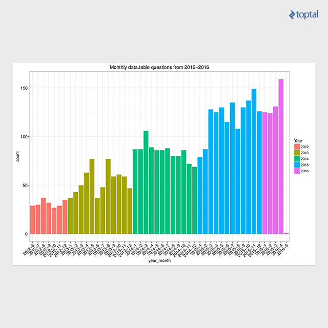
There are plenty of resources available. Besides the manuals available for each function, there are also package vignettes, which are tutorials focused around the particular subject. 这些可以在 开始 page. 此外, 演讲 page lists more than 30 materials (slides, video, etc.) from data.table presentations around the globe. Also, the community support has grown over the years, recently reaching the 4000-th question on Stack Overflow data.table tag, still having a high ratio (91.9%)的回答问题. The below plot presents the number of data.table tagged questions on Stack Overflow over time.
This article provides chosen examples for efficient tabular data transformation in R using the data.table package. The actual figures on performance can be examined by looking for reproducible benchmarks. I published a summarized blog post about data.table solutions for the top 50 rated StackOverflow questions for R语言 called Solve common R problems efficiently with data.table, where you can find a lot of figures and reproducible code. 这个包 data.table uses native implementation of fast radix ordering for its grouping operations, and binary search for fast subsets/joins. This radix ordering has been incorporated into base R from version 3.3.0. 此外, algorithm was recently implemented into H2O machine learning platform and parallelized over H2O cluster, enabling efficient big joins on 10B x 10B rows.
World-class articles, delivered weekly.
World-class articles, delivered weekly.